网页网站制作公司宁波网站推广哪家公司好
参考文献
PINN(Physics-informed Neural Networks)的原理部分可参见https://maziarraissi.github.io/PINNs/
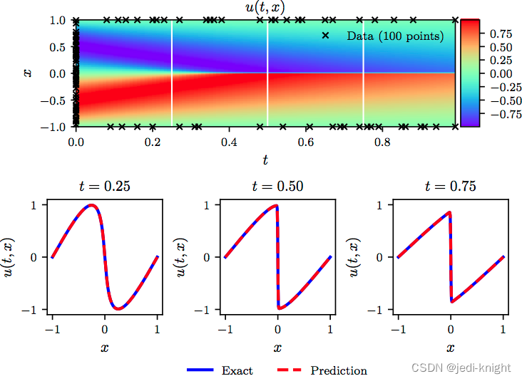
考虑Burgers方程,如下图所示,初始时刻u符合sin分布,随着时间推移在x=0处发生间断.
这是一个经典问题,可使用pytorch通过PINN实现对Burgers方程的求解。
源代码与注释
源代码共含有三个文件,来源于Github https://github.com/jayroxis/PINNs

network.py文件用于定义神经网络的结构
train.py文件用于训练神经网络
evaluate.py文件用于测试训练好的模型绘制结果图
建议使用Anaconda构建运行环境,需要安装pytorch和一些辅助包。
1、network.py 文件
import torch
import torch.nn as nn
from collections import OrderedDict# 定义神经网络的架构
class Network(nn.Module):# 构造函数def __init__(self,input_size, # 输入层神经元数hidden_size, # 隐藏层神经元数output_size, # 输出层神经元数depth, # 隐藏层数act=torch.nn.Tanh, # 输入层和隐藏层的激活函数):super(Network, self).__init__()#调用父类的构造函数# 输入层layers = [('input', torch.nn.Linear(input_size, hidden_size))]layers.append(('input_activation', act()))# 隐藏层for i in range(depth):layers.append(('hidden_%d' % i, torch.nn.Linear(hidden_size, hidden_size)))layers.append(('activation_%d' % i, act()))# 输出层layers.append(('output', torch.nn.Linear(hidden_size, output_size)))#将这些层组装为神经网络self.layers = torch.nn.Sequential(OrderedDict(layers))# 前向计算方法def forward(self, x):return self.layers(x)
2、train.py 文件
import math
import torch
import numpy as np
from network import Network# 定义一个类,用于实现PINN(Physics-informed Neural Networks)
class PINN:# 构造函数def __init__(self):# 选择使用GPU还是CPUdevice = torch.device("cuda") if torch.cuda.is_available() else torch.device("cpu")# 定义神经网络self.model = Network(input_size=2,  # 输入层神经元数hidden_size=16,  # 隐藏层神经元数output_size=1,  # 输出层神经元数depth=8,  # 隐藏层数act=torch.nn.Tanh  # 输入层和隐藏层的激活函数).to(device)  # 将这个神经网络存储在GPU上(若GPU可用)self.h = 0.1  # 设置空间步长self.k = 0.1  # 设置时间步长x = torch.arange(-1, 1 + self.h, self.h)  # 在[-1,1]区间上均匀取值,记为xt = torch.arange(0, 1 + self.k, self.k)  # 在[0,1]区间上均匀取值,记为t# 将x和t组合,形成时间空间网格,记录在张量X_inside中self.X_inside = torch.stack(torch.meshgrid(x, t)).reshape(2, -1).T# 边界处的时空坐标bc1 = torch.stack(torch.meshgrid(x[0], t)).reshape(2, -1).T  # x=-1边界bc2 = torch.stack(torch.meshgrid(x[-1], t)).reshape(2, -1).T  # x=+1边界ic = torch.stack(torch.meshgrid(x, t[0])).reshape(2, -1).T  # t=0边界self.X_boundary = torch.cat([bc1, bc2, ic])  # 将所有边界处的时空坐标点整合为一个张量# 边界处的u值u_bc1 = torch.zeros(len(bc1))  # x=-1边界处采用第一类边界条件u=0u_bc2 = torch.zeros(len(bc2))  # x=+1边界处采用第一类边界条件u=0u_ic = -torch.sin(math.pi * ic[:, 0])  # t=0边界处采用第一类边界条件u=-sin(pi*x)self.U_boundary = torch.cat([u_bc1, u_bc2, u_ic])  # 将所有边界处的u值整合为一个张量self.U_boundary = self.U_boundary.unsqueeze(1)# 将数据拷贝到GPUself.X_inside = self.X_inside.to(device)self.X_boundary = self.X_boundary.to(device)self.U_boundary = self.U_boundary.to(device)self.X_inside.requires_grad = True  # 设置:需要计算对X的梯度# 设置准则函数为MSE,方便后续计算MSEself.criterion = torch.nn.MSELoss()# 定义迭代序号,记录调用了多少次lossself.iter = 1# 设置lbfgs优化器self.lbfgs = torch.optim.LBFGS(self.model.parameters(),lr=1.0,max_iter=50000,max_eval=50000,history_size=50,tolerance_grad=1e-7,tolerance_change=1.0 * np.finfo(float).eps,line_search_fn="strong_wolfe",)# 设置adam优化器self.adam = torch.optim.Adam(self.model.parameters())# 损失函数def loss_func(self):# 将导数清零self.adam.zero_grad()self.lbfgs.zero_grad()# 第一部分loss: 边界条件不吻合产生的lossU_pred_boundary = self.model(self.X_boundary)  # 使用当前模型计算u在边界处的预测值loss_boundary = self.criterion(U_pred_boundary, self.U_boundary)  # 计算边界处的MSE# 第二部分loss:内点非物理产生的lossU_inside = self.model(self.X_inside)  # 使用当前模型计算内点处的预测值# 使用自动求导方法得到U对X的导数du_dX = torch.autograd.grad(inputs=self.X_inside,outputs=U_inside,grad_outputs=torch.ones_like(U_inside),retain_graph=True,create_graph=True)[0]du_dx = du_dX[:, 0]  # 提取对第x的导数du_dt = du_dX[:, 1]  # 提取对第t的导数# 使用自动求导方法得到U对X的二阶导数du_dxx = torch.autograd.grad(inputs=self.X_inside,outputs=du_dX,grad_outputs=torch.ones_like(du_dX),retain_graph=True,create_graph=True)[0][:, 0]loss_equation = self.criterion(du_dt + U_inside.squeeze() * du_dx, 0.01 / math.pi * du_dxx)  # 计算物理方程的MSE# 最终的loss由两项组成loss = loss_equation + loss_boundary# loss反向传播,用于给优化器提供梯度信息loss.backward()# 每计算100次loss在控制台上输出消息if self.iter % 100 == 0:print(self.iter, loss.item())self.iter = self.iter + 1return loss# 训练def train(self):self.model.train()  # 设置模型为训练模式# 首先运行5000步Adam优化器print("采用Adam优化器")for i in range(5000):self.adam.step(self.loss_func)# 然后运行lbfgs优化器print("采用L-BFGS优化器")self.lbfgs.step(self.loss_func)# 实例化PINN
pinn = PINN()# 开始训练
pinn.train()# 将模型保存到文件
torch.save(pinn.model, 'model.pth')
运行该文件后模型结果保存在model.pth文件中
3、evaluate.py 文件
import torch
import seaborn as sns
import matplotlib.pyplot as plt# 选择GPU或CPU
device = torch.device("cuda") if torch.cuda.is_available() else torch.device("cpu")# 从文件加载已经训练完成的模型
model_loaded = torch.load('model.pth', map_location=device)
model_loaded.eval() # 设置模型为evaluation状态# 生成时空网格
h = 0.01
k = 0.01
x = torch.arange(-1, 1, h)
t = torch.arange(0, 1, k)
X = torch.stack(torch.meshgrid(x, t)).reshape(2, -1).T
X = X.to(device)# 计算该时空网格对应的预测值
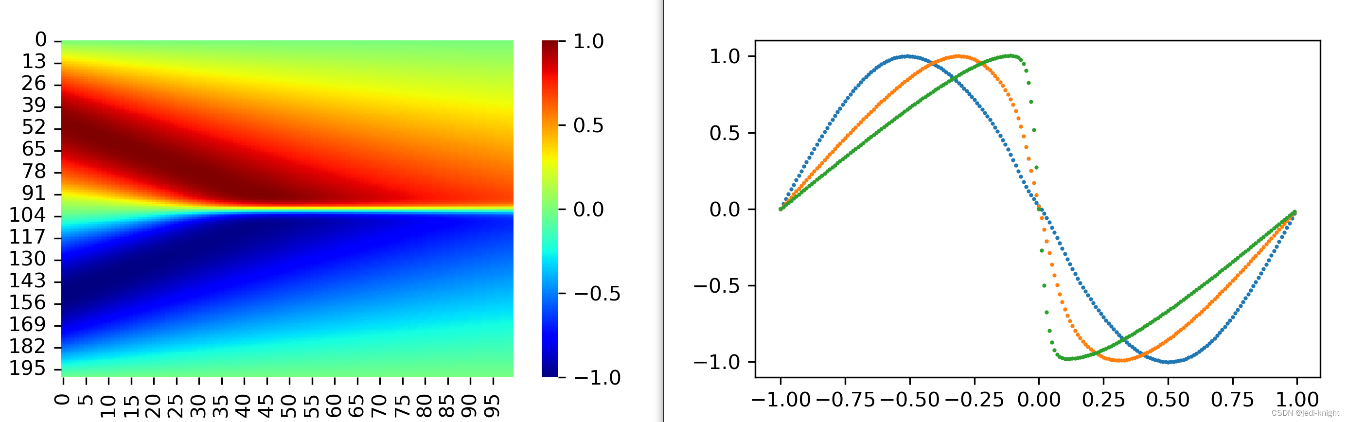
with torch.no_grad():U_pred = model_loaded(X).reshape(len(x), len(t)).cpu().numpy()# 绘制计算结果
plt.figure(figsize=(5, 3), dpi=300)
xnumpy = x.numpy()
plt.plot(xnumpy, U_pred[:, 0], 'o', markersize=1)
plt.plot(xnumpy, U_pred[:, 20], 'o', markersize=1)
plt.plot(xnumpy, U_pred[:, 40], 'o', markersize=1)
plt.figure(figsize=(5, 3), dpi=300)
sns.heatmap(U_pred, cmap='jet')
plt.show()
运行该文件后,可绘制u场的结果